Ideal Rankine Cycle with reheat calculations

The problem

Consider a reheat cycle utilizing steam. Steam leaves the boiler and enters the turbine at 4 MPa, 400\(^\circ\)C. After expansion in the turbine to 400 kPa, the steam is reheated to 400\(^\circ\)C and then expanded in the low-pressure turbine to 10 kPa. Determine the cycle efficiency.

Initiate PYroMat and configure its units:

import pyromat as pm

pm.config["unit_pressure"] = "kPa"
pm.config["def_p"] = 100

mp_water = pm.get("mp.H2O") # <-- for multi-phase water properties

To solve this problem we consider a control surface around the pump, the boiler, the turbine, and the condenser.

The pump

First, consider the pump:

#saturated liquid, thus x = 0
p1 = 10
s1 = mp_water.ss(p=p1)[0]
T1 = mp_water.Ts(p=p1)[0]

p2 = 4000
s2 = s1
T2 = mp_water.T_h(h=h2,p=p2)

h2dash = mp_water.hs(p=p2)[0]
s2dash = mp_water.ss(p=p2)[0]
T2dash = mp_water.Ts(p=p2)[0]

h3dash = mp_water.hs(p=p2)[1]
s3dash = mp_water.ss(p=p2)[1]
T3dash = T2dash

v = 1/mp_water.ds(p=p1)[0]

w_p = v*(p2-p1)

print(f"Specific volume: {round(float(v),5)} m^3/kg")
print(f"Work required by pump: {round(float(w_p),1)} kJ/kg")

Specific volume: 0.00101 m^3/kg
Work required by pump: 4.0 kJ/kg

h1 = mp_water.hs(p=p1)[0]
h2 = h1+w_p
print(f"h2 = {round(float(h2),1)} kJ/kg")

h2 = 195.8 kJ/kg

The HP turbine

Next, let’s consider the high pressure turbine:

p3 = p2
T3 = 400 + 273.15
h3 = mp_water.h(p=p3, T=T3)
s3 = mp_water.s(p=p3, T=T3)

p4 = 400
s4 = s3
T4, x4 = mp_water.T_s(s=s4, p=p4, quality=True)
h4 = mp_water.h(x=x4, p=p4)

w_HPt = h3-h4

print(f"Quality of intermediate pressure steam: {round(float(x4),4)}")
print(f"Work generated by HP turbine: {round(float(w_HPt),1)} kJ/kg")

Quality of intermediate pressure steam: 0.9757
Work generated by HP turbine: 528.2 kJ/kg

The LP turbine

Now, we consider the low pressure turbine:

p5 = p4
T5 = 400 + 273.15 
h5 = mp_water.h(p=p5, T=T5)
s5 = mp_water.s(p=p5, T=T5)

p6 = p1
s6 = s5

T6, x6 = mp_water.T_s(s=s6, p=p6, quality=True)
h6 = mp_water.h(x=x6, p=p6)

w_LPt = h5-h6

print(f"Quality of low pressure steam: {round(float(x6),4)}")
print(f"Work generated by LP turbine: {round(float(w_LPt),1)} kJ/kg")
print(f"Total work output by turbine: {round(float(w_HPt+w_LPt),1)} kJ/kg")

Quality of low pressure steam: 0.9669
Work generated by LP turbine: 769.3 kJ/kg
Total work output by turbine: 1297.5 kJ/kg

The boiler

Next, let’s consider the boiler:

q_H = (h3-h2)+(h5-h4)
print(f"Heat input by boiler: {round(float(q_H),1)} kJ/kg")

Heat input by boiler: 3606.2 kJ/kg

The condenser

Finally, we consider the condenser:

q_L = h6-h1
print(f"Heat rejected by the condenser: {round(float(q_L),1)} kJ/kg")

Heat rejected by the condenser: 2312.8 kJ/kg

Calculating the thermal efficiency

We can now calculate the thermal efficiency with \[\eta_{th}=\frac{w_{net}}{q_H}\]

eta_th = (w_HPt+w_LPt-w_p)/q_H*100
print(f"Thermal efficiency is: {round(float(eta_th),1)}%")

Thermal efficiency is: 35.9%

The Rankine cycle on a graph

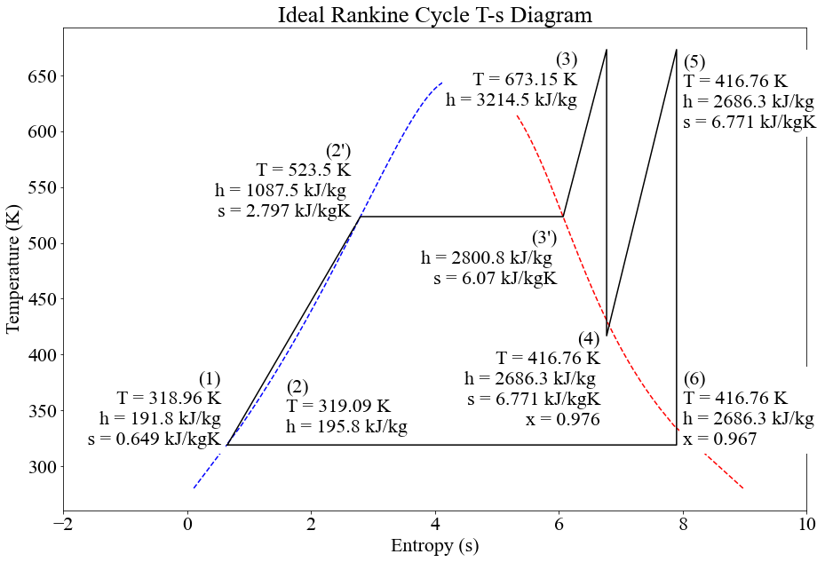
Once all the values have been calculated, the ideal Rankine Cycle can be shown visually with the use of a graph.

import numpy as np
import matplotlib.pyplot as plt

p = np.linspace(1,22063,1000)
T = mp_water.Ts(p=p)
s = mp_water.ss(p=p)


font = {'family' : 'Times New Roman',
        'size'   : 22}


plt.figure(figsize=(15,10))
plt.title('Ideal Rankine Cycle T-s Diagram')
plt.rc('font', **font)
plt.plot(s[0],T, 'b--')
plt.plot(s[1],T,'r--')
plt.ylabel('Temperature (K)')
plt.xlabel('Entropy (s)')
plt.xlim(-2,10)
#plt.ylim(200,800)
plt.plot([s1, s2, s2dash, s3dash, s3, s4, s5, s6, s1],[T1, T2, T2dash, T3dash, T3, T4, T5, T6, T1], 'black')

plt.text(s1-.1,T1,f'(1)\nT = {round(float(T1),2)} K\nh = {round(float(h1),1)} kJ/kg\n s = {round(float(s1),3)} kJ/kgK',
    ha='right',backgroundcolor='white')
plt.text(1.6,330,f'(2)\nT = {round(float(T2),2)} K\nh = {round(float(h2),1)} kJ/kg',
    ha='left',backgroundcolor='white')
plt.text(s2dash-.15,T2dash,f"(2')\nT = {round(float(T2dash),2)} K\nh = {round(float(h2dash),1)} kJ/kg \ns = {round(float(s2dash),3)} kJ/kgK",
    ha='right',backgroundcolor='white')
plt.text(s3dash-.1,T3dash-60,f"(3')\nh = {round(float(h3dash),1)} kJ/kg \ns = {round(float(s3dash),3)} kJ/kgK",
    ha='right',backgroundcolor='white')
plt.text(6.3,T3-50,f'(3)\nT = {round(float(T3),2)} K\nh = {round(float(h3),1)} kJ/kg',
    ha='right',backgroundcolor='white')
plt.text(s4-.1,T4-80,f'(4)\nT = {round(float(T4),2)} K\nh = {round(float(h4),1)} kJ/kg \ns = {round(float(s4),3)} kJ/kgK\nx = {round(float(x4),3)}',
    ha='right',backgroundcolor='white')
plt.text(s5+.1,T5-70,f'(5)\nT = {round(float(T4),2)} K\nh = {round(float(h4),1)} kJ/kg \ns = {round(float(s4),3)} kJ/kgK',
    ha='left',backgroundcolor='white')
plt.text(s6+.1,T6,f'(6)\nT = {round(float(T4),2)} K\nh = {round(float(h4),1)} kJ/kg \nx = {round(float(x6),3)}',
    ha='left',backgroundcolor='white')